

Model Experimentation: End-to-End SiteEUI-Prediction with Explainability using Kubeflow Notebooks.

Hey I'm Samiksha Kolhe. a Data Enthusiast and aspiring Data Scientist. One day Fascinated by a fact that "We can built Time machines and predict future using AI". That hit my dream to explore the Vector space and find out what the dark matter is about. World and Technology every day brings new challenges, and new learnings. Technology fascinated me, I'm constantly seeking out new challenges and opportunities to learn and grow. A born-ready girl with deep expertise in ML, Data Science, and Deep Learning, generative AI. Curious & Self-learner with a go-getter attitude that pushes me to build things. My passion lies in solving business problems with the help of Data. Love to solve customer-centric problems. Retail, fintech, e-commerce businesses to solve the customer problems using Data/AI. Currently learning MLops to build robust Data/ML systems for production-ready applications. exploring GenAI. As a strong collaborator and communicator, I believe in the power of teamwork and diversity of thoughts to solve a problem. I'm always willing to lend a helping hand to my colleagues and juniors. Through my Hashnode blog, I share my insights, experiences, and ideas with the world. I love to writing about latest trends in AI and help students/freshers to start in their AI journey. Outside technology I'm a spiritual & Yoga person. Help arrange Yoga and mediation campaigns, Volunteering to contribute for better society. Love Travelling, Reading and Learn from world.
Hello Techies!!👋 Hope you all doing Amazing. I come up with another article on kubeflow. if you're new to this article and kubeflow. check out my previous article here, where I explained in detail information about the kubeflow tool and setup on Amazon EC-2.
This Article is medium to advanced level for those who have some knowledge of ML model lifecycle and regression problems.
In this article, I've explained how to launch your first kubeflow notebook and ML model experimentation using the Site-Energy utility intensity prediction regression Problem.
Note: I've provided the best of industry materials under each section which you can use to learn and practice each component of the ML model lifecycle. So, Don't forget to click on the links:)
wait wait.. As a Bonus!! Explained how Model Explainability can be interpreted and used using the SHAP library.
Excited!! Let's see Our Agenda first
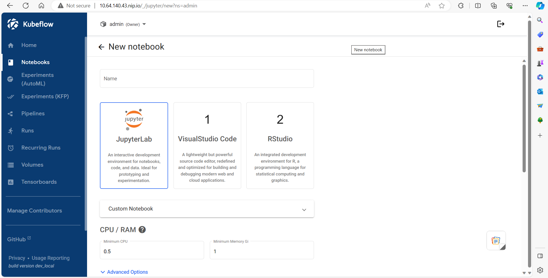
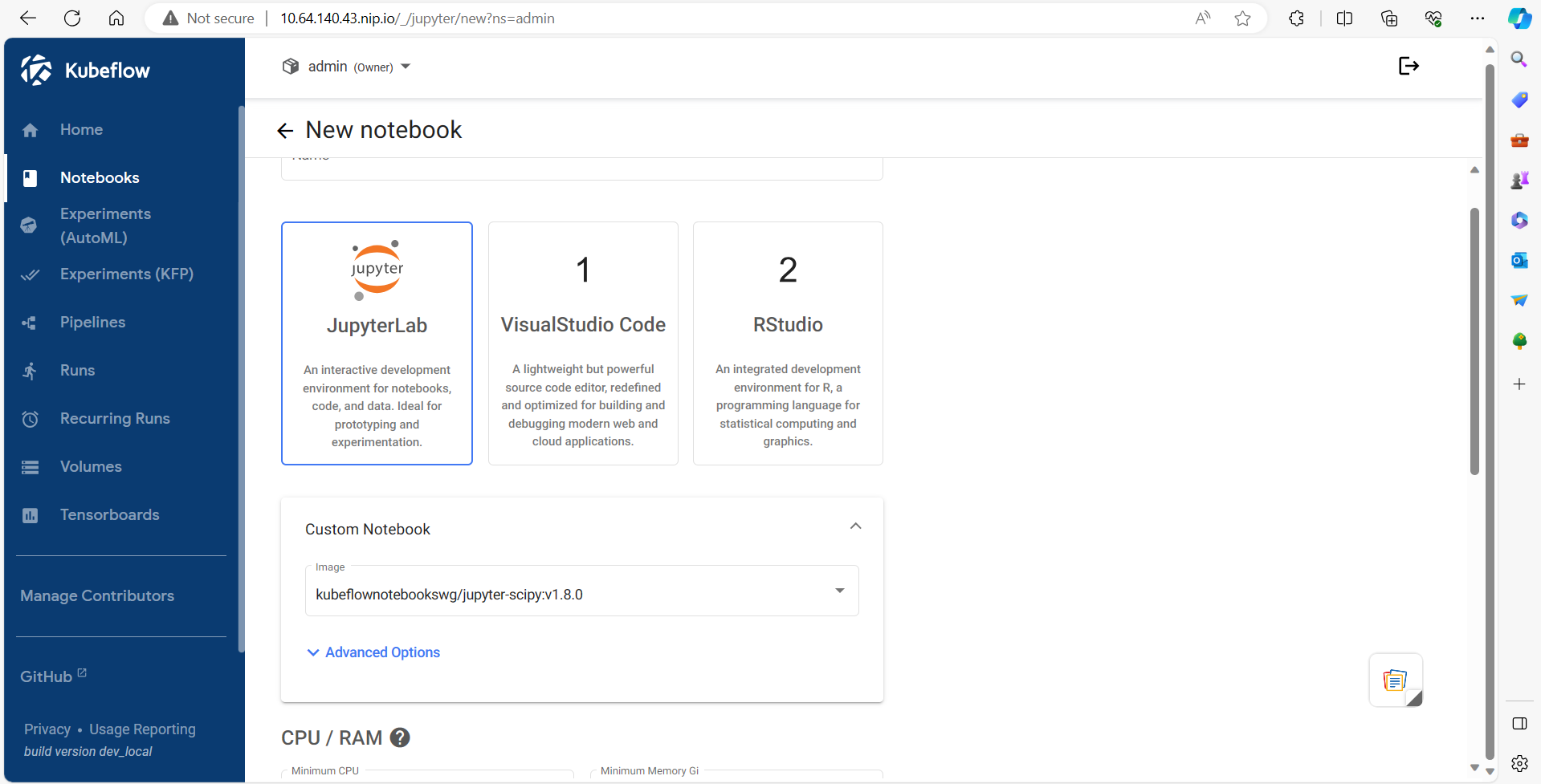
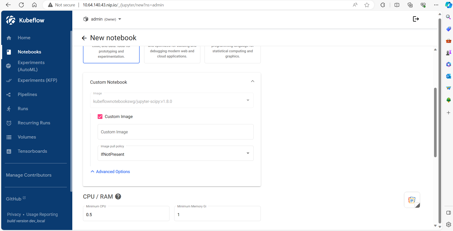
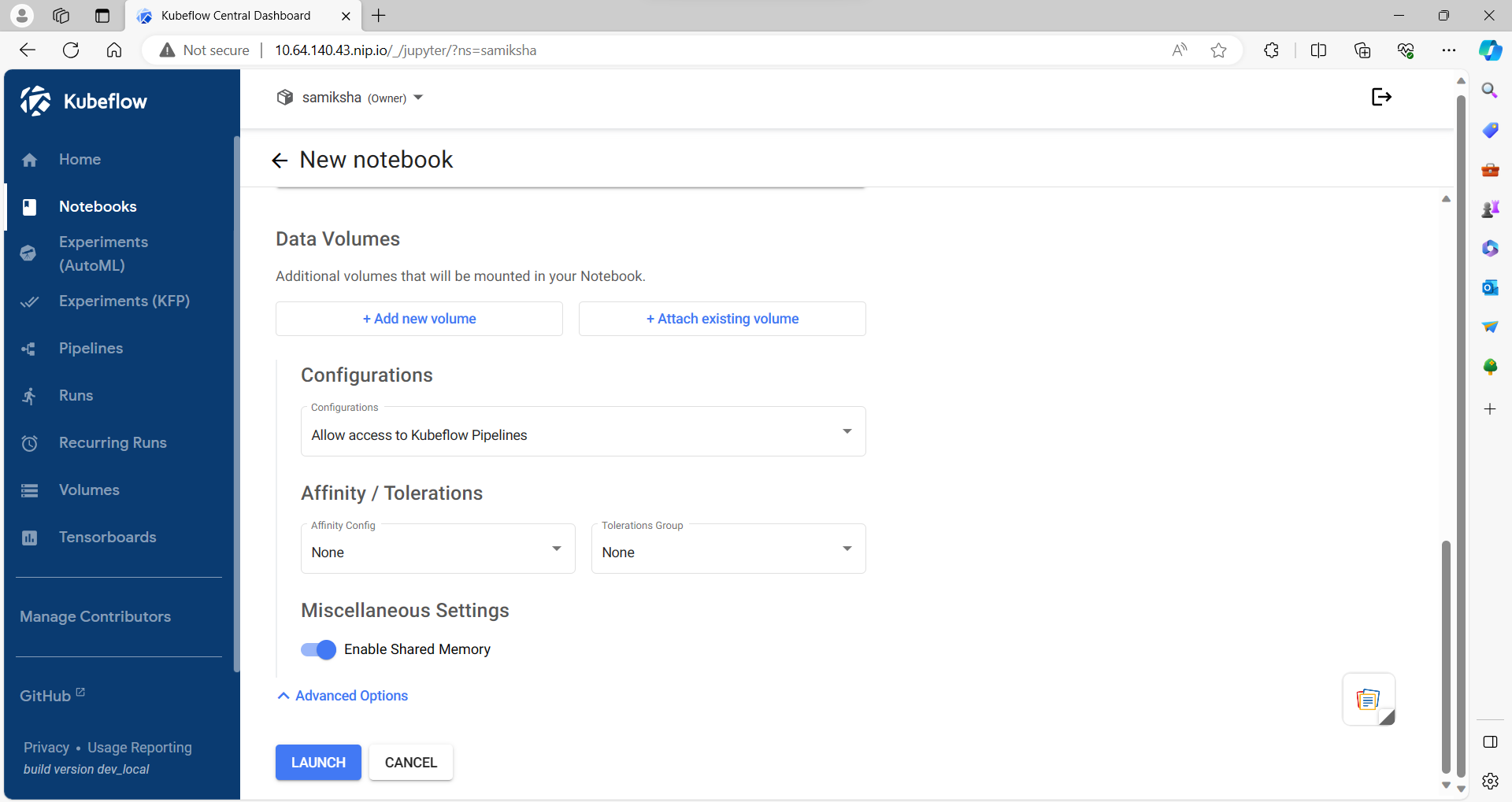
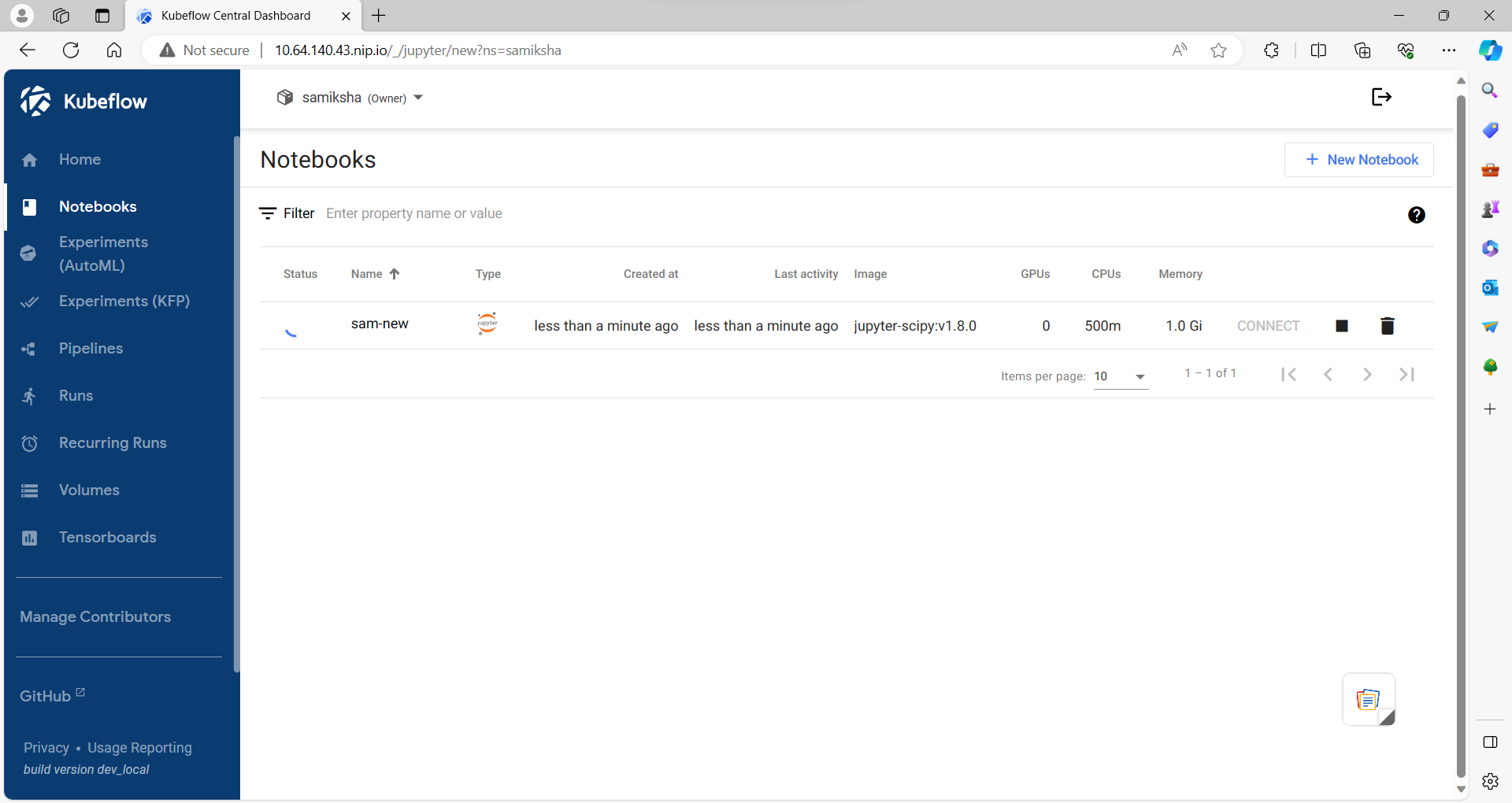
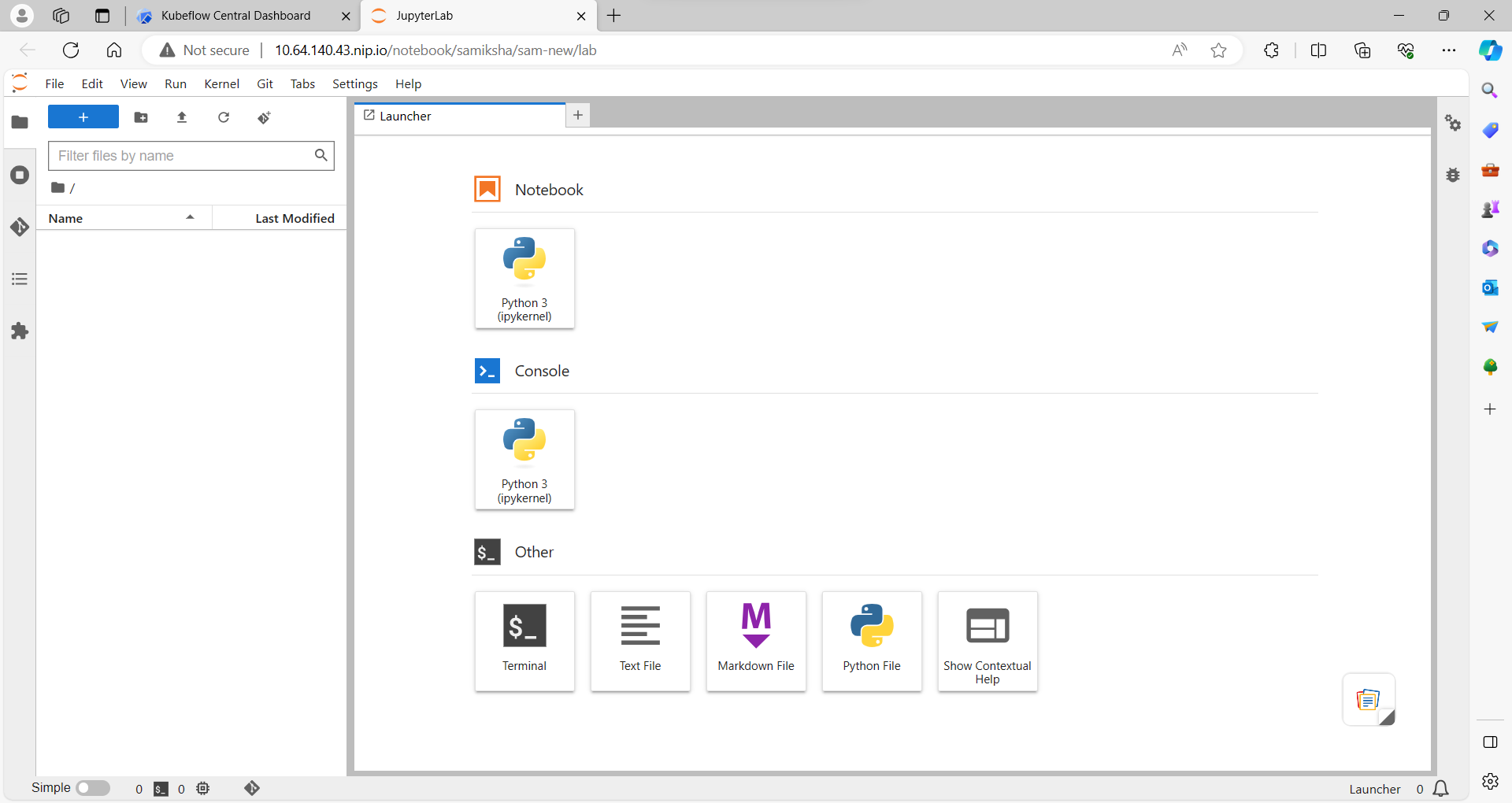
Launch Kubeflow Notebook
Data Importing using Minio
Exploratory Data Analysis
Data Preprocessing/wrangling
Feature Engineering
Feature Scaling
Model Experimentation
Hyperparameter training using Optuna
Best Model Selection and Testing.
Model Explainability using SHAP.
Let's get started🤩
1. Launch Kubeflow Notebook

2.Data Importing using Minio
More about Data collection🤩
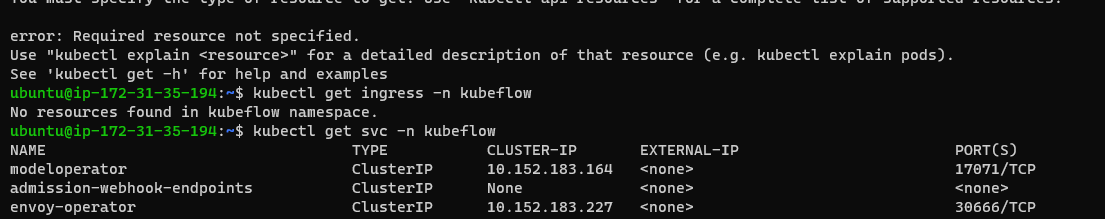
In order to provide a single source of truth where all your working data (training and testing data, saved ML models etc.) is available to all your components, using an object storage is a recommended way. For our app, we will setup MinIO.
Since Kubeflow has already setup a MinIO tenant, we will leverage the mlpipeline bucket. But you can also deploy your own MinIO tenant.
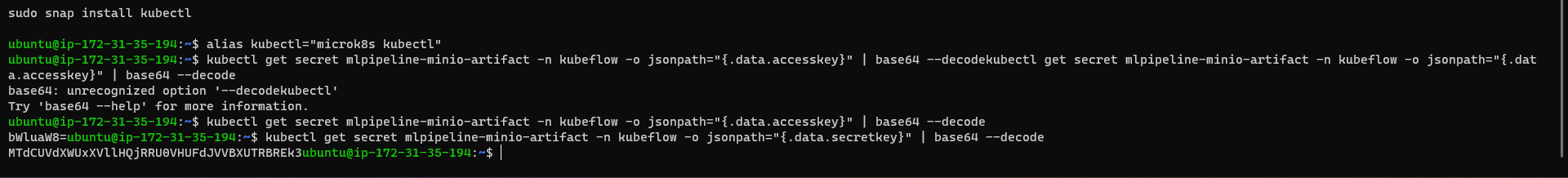
Get credentials from Kubeflow's integrated MinIO
- Obtain the accesskey and secretkey for MinIO with these commands:
kubectl get secret mlpipeline-minio-artifact -n kubeflow -o jsonpath="{.data.accesskey}" | base64 --decode
kubectl get secret mlpipeline-minio-artifact -n kubeflow -o jsonpath="{.data.secretkey}" | base64 --decode

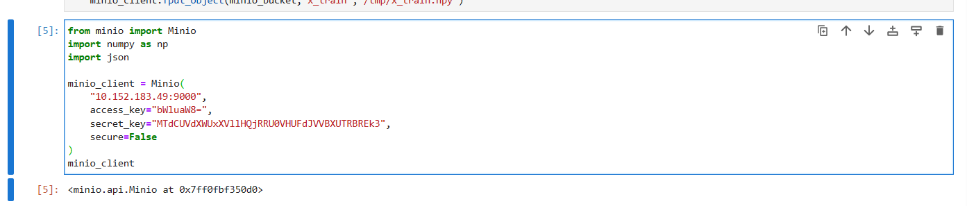
This is how you can setup minio as an object storage as default available on microk8s. here is the complete guide by which you can get and put the data into minio.
Without going into fetching and putting data into your s3 storage. let's understand the model pipeline in detail further.
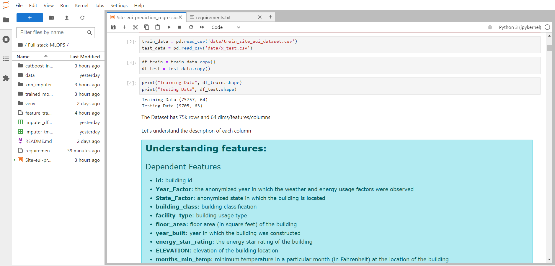
Let's start Model experimentation🔁, below I've built an end-to-end machine learning project, where I tried to explain how a machine learning project should be built, the ML project lifecycle and what are the necessary steps to be followed for Robust Model building.
Note: in-detail code is not explained below but The notebook Code and Data are available here. Notebook-Code, Github-code & Site-EUI-data. You can import the notebook.
Let's get started🤩
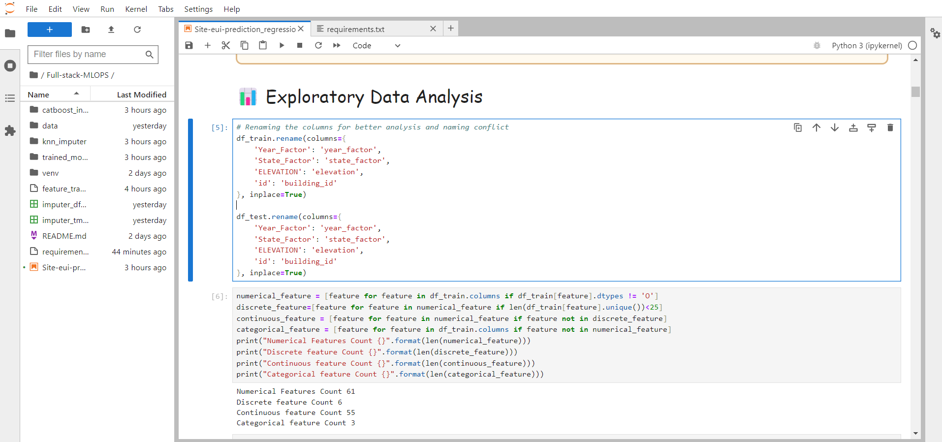
3. Exploratory Data Analysis
Exploratory Data Analysis is the first step in understanding your data and acquiring domain knowledge. It helps in knowing the real features apart. Perform EDA using the following resources and note down your insights with the most visualizations that you perform.
Imagine EDA as detective work for your data. We use tools like charts and graphs to unveil the story hidden in the numbers. Think of it like checking the health of your dataset by looking for patterns and weird things. This helps us understand what we're working with before jumping into the real action.
EDA is all about getting to know about all features, correlation, multi-collinearity, relations between independent features and target data, outliers, data distribution, handling missing values, Feature Encoding, imbalance-data treatment etc. To prepare for further lifecycle steps.
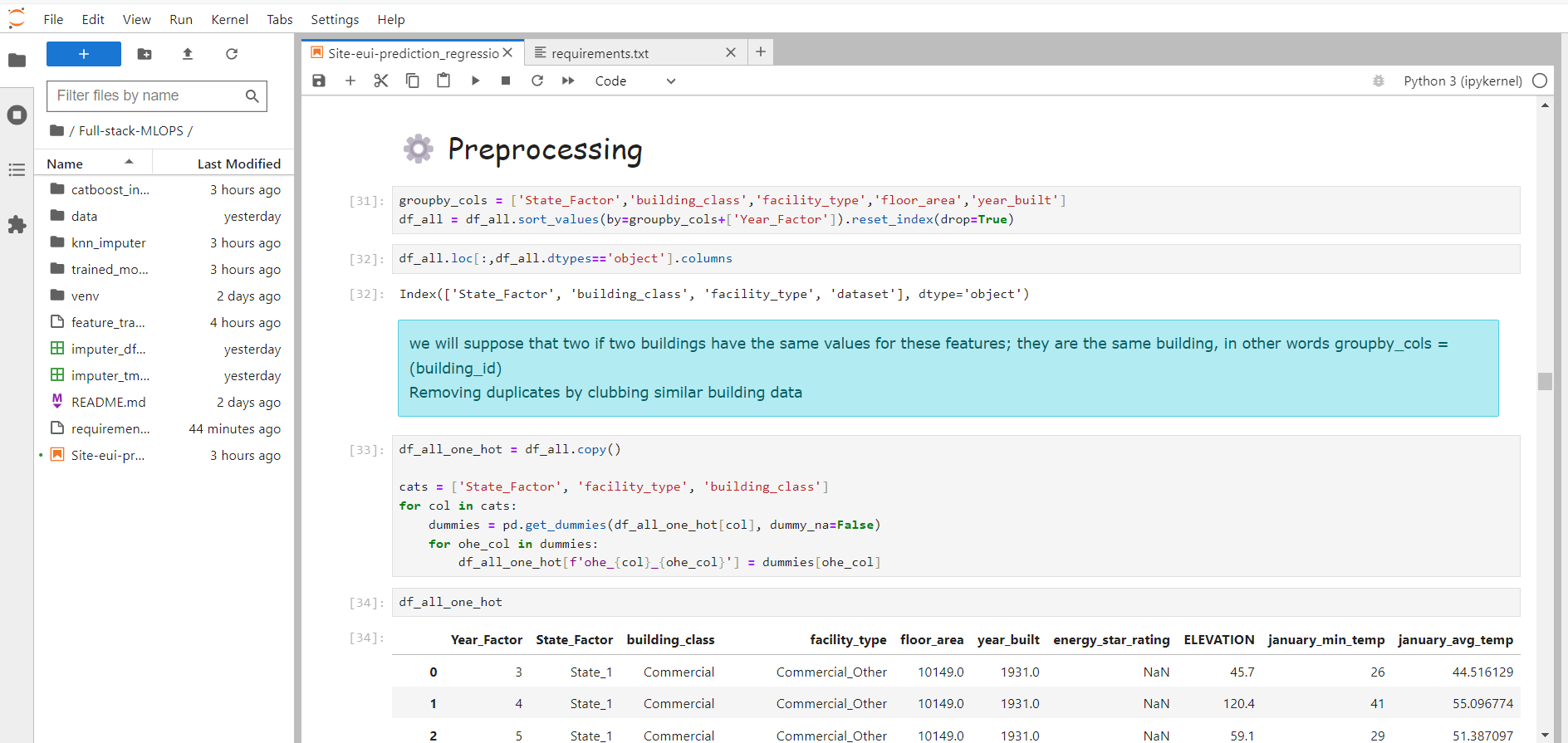
4. Data Preprocessing/Wrangling
More on Data preprocessing..
It's about applying the finding during EDA on to the data.
Now, let's tidy up our data. It's like cleaning your room before starting homework. We deal with missing values, turn words into numbers, and handle any weird numbers that might mess up our predictions. This step ensures our data is neat and ready for the machine to learn.
Handling Missing Data:
Identify and analyze missing values in the dataset.
Options for handling missing data include removing rows/columns, imputing values using statistical measures (mean, median, mode), or using more advanced imputation techniques.
Dealing with Duplicate Data:
- Identify and remove duplicate records if any. Duplicates can skew analysis and modeling results.
Encoding Categorical Variables:
- Convert categorical variables (like gender or product categories) into numerical representations. Common methods include one-hot encoding, label encoding, or binary encoding.
Handling Outliers:
- Identify and handle outliers, which are data points significantly different from the majority. Outliers can impact the performance of machine learning models. Techniques include truncation, transformation, or imputation.
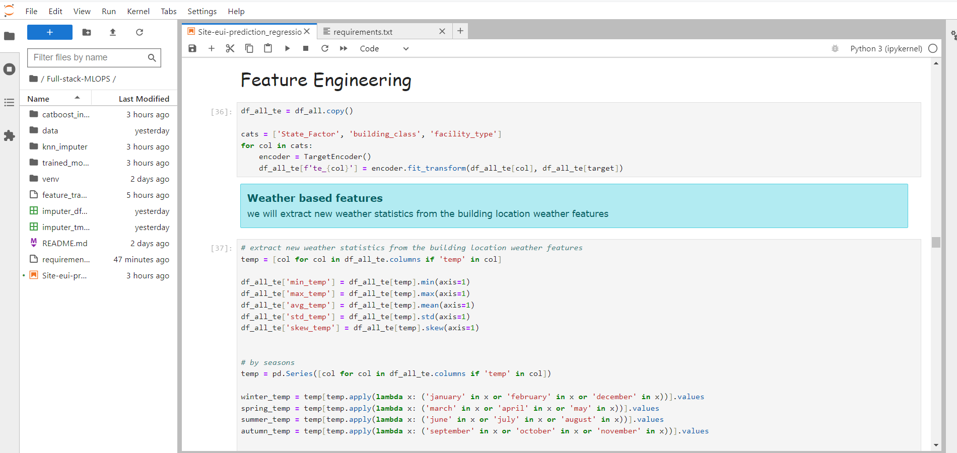
5. Feature Engineering
More about Feature Engineering
This is where we get creative with our data. Feature engineering is like giving your machine learning model superpowers. We create new features or tweak existing ones to help our model understand the problem better. It's about making our data more useful for prediction.
Domain Understanding:
- Gain a deep understanding of the problem domain and the specific characteristics of the data. This helps in identifying relevant features that could have a significant impact on the model's performance.
Handling Date and Time Features:
- Extract meaningful information from date and time features, such as day of the week, month, or time intervals. This can provide additional insights for the model.
Feature Importance Analysis:
- Use techniques like feature importance from tree-based models to identify the most influential features. Focus on these features during the modeling process.
Dimensionality Reduction:
- If dealing with high-dimensional data, consider techniques like Principal Component Analysis (PCA) to reduce the number of features while retaining essential information.
Custom Feature Creation:
- Create a new feature based on previous features available.
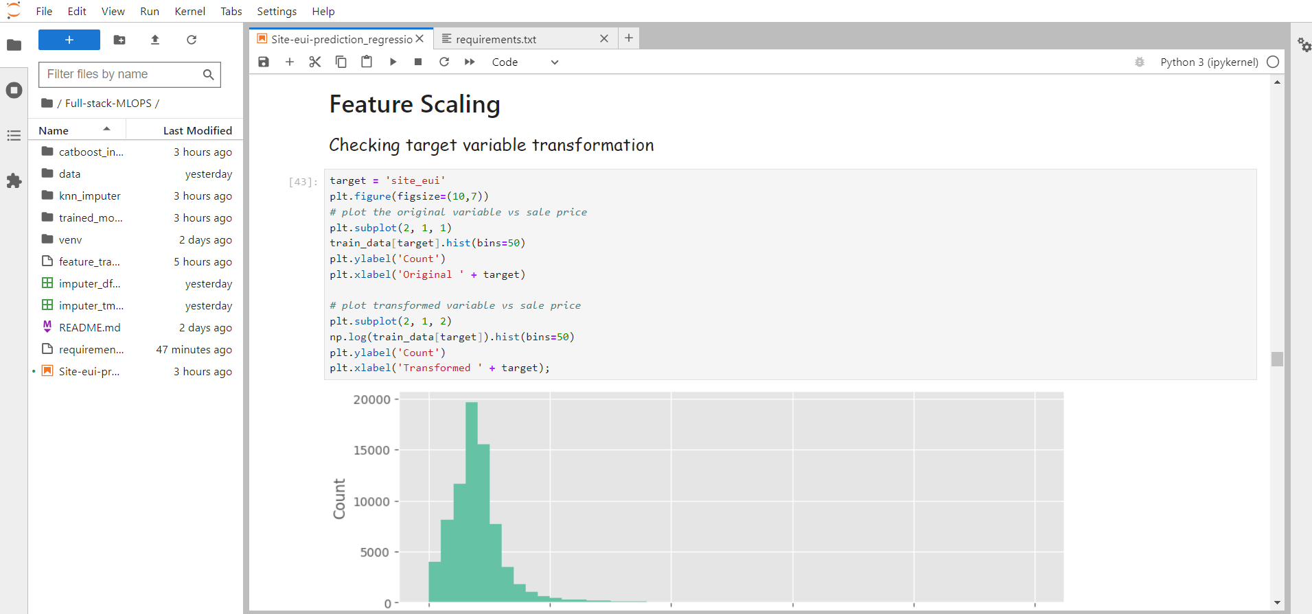
6. Feature Scaling
More about Feature Scaling
Machines don't always understand big and small in the same way we do. Feature scaling is like making sure everyone speaks the same language. We want our features to be on a level playing field so that no one dominates the conversation.
Min-Max Scaling (Normalization):
- Scales the features to a specific range, typically [0, 1].
Standardization (Z-score normalization):
- Transforms the features to have a mean of 0 and a standard deviation of 1.
Robust Scaling:
- Scales features based on the interquartile range (IQR) to make them robust to outliers.It is especially useful when the data contains outliers.
Log Transformation:
- Applies a logarithmic function to the features, which can help when the original data has a skewed distribution.
Power Transformations:
- Apply power transformations like square root, cube root, or Box-Cox to stabilize variance and make the distribution more Gaussian.
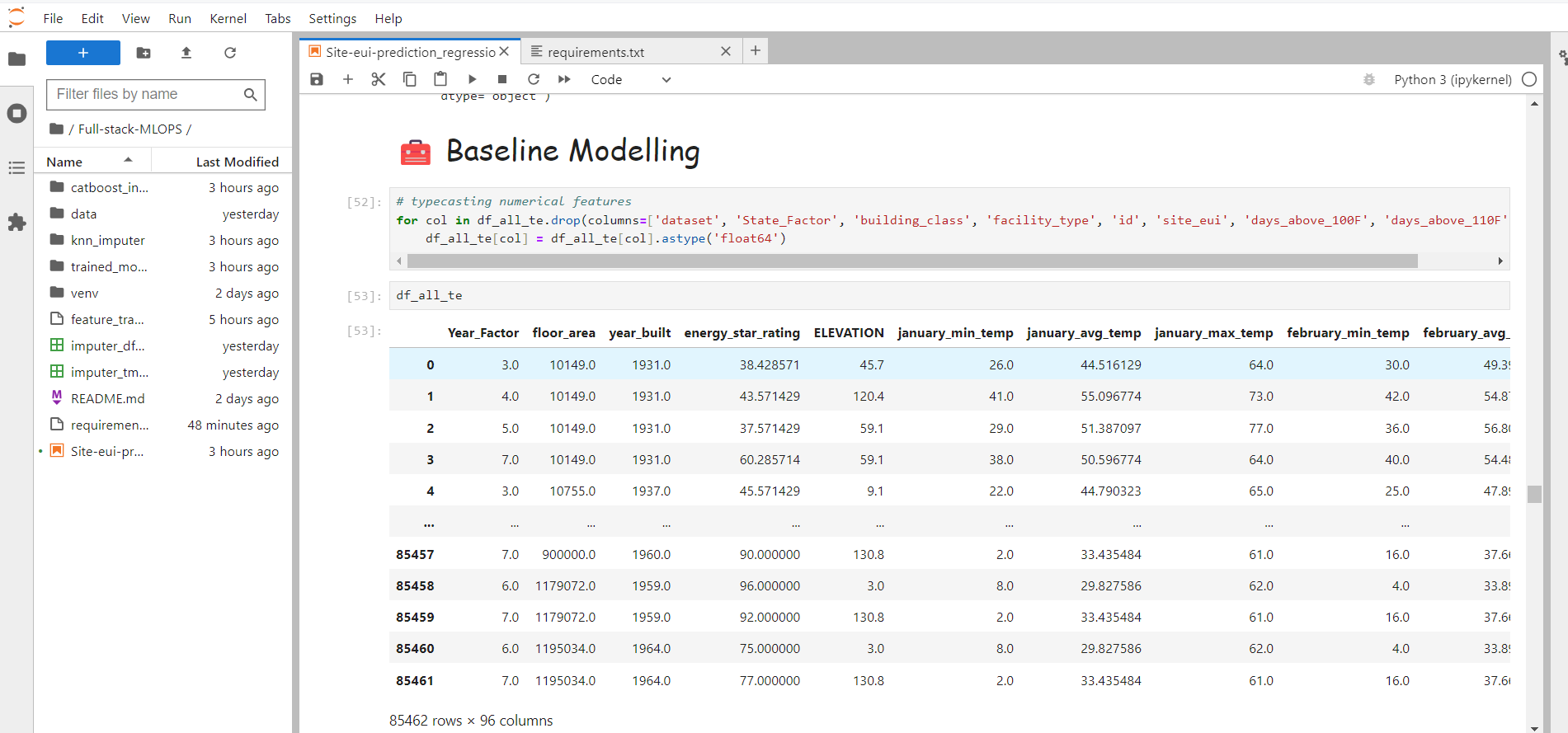
7. Model Experimentation
Time to pick a tool for the job! We have a bunch of algorithms (fancy word for methods) to choose from, like picking the right tool from a toolbox. Linear regression, decision trees, and friends are here to help us make predictions. Each has its strengths, so we choose based on the problem we're solving.
Model experimentation involves choosing the right model based on previous Data analysis, to best fit our data by considering and handling the bias-variance trade-off.
in this project as it's a regression problem, tried Linear algorithms like Lasso regression, Boosting algorithm like Xgboost[Xtremely flexible and best to use], Catboost, bagging algorithms like Random Forest etc.
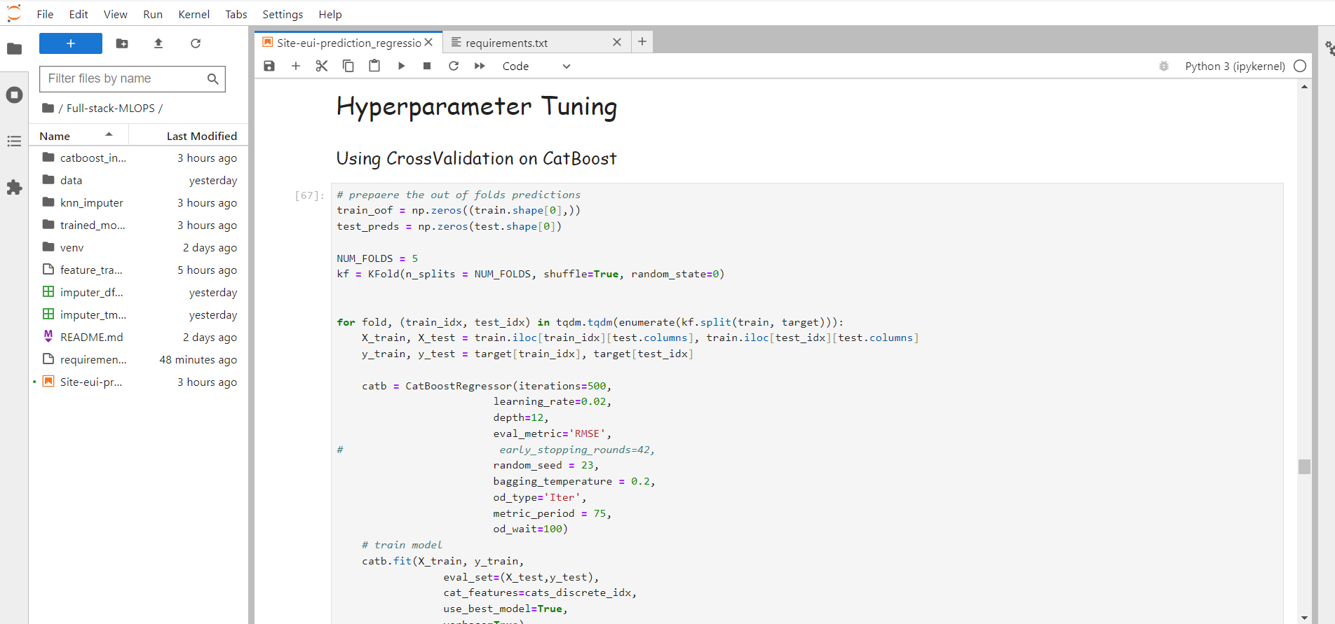
8. Hyperparameter tuning using Optuna
More about model tuning/optuna
Picture this as adjusting the knobs on your music system until the sound is just right. In machine learning, we tweak the settings of our model to make it perform its best. It's a bit like finding the perfect recipe – we adjust until our model tastes success!
After choosing the best set of models, we can do further cross-validation as it's a regularisation method to handle imbalanced data and overfitting problems.

9. Best Model Selection and Testing
Model building is an iterative Process. which technique will best suit which data can be concluded only after a lot of model experimentation. But at the End whichever model performs best not in terms of Low Error or more accuracy, in every aspect of model evaluation/error distribution/overfitting/data leakage etc. is chosen for production
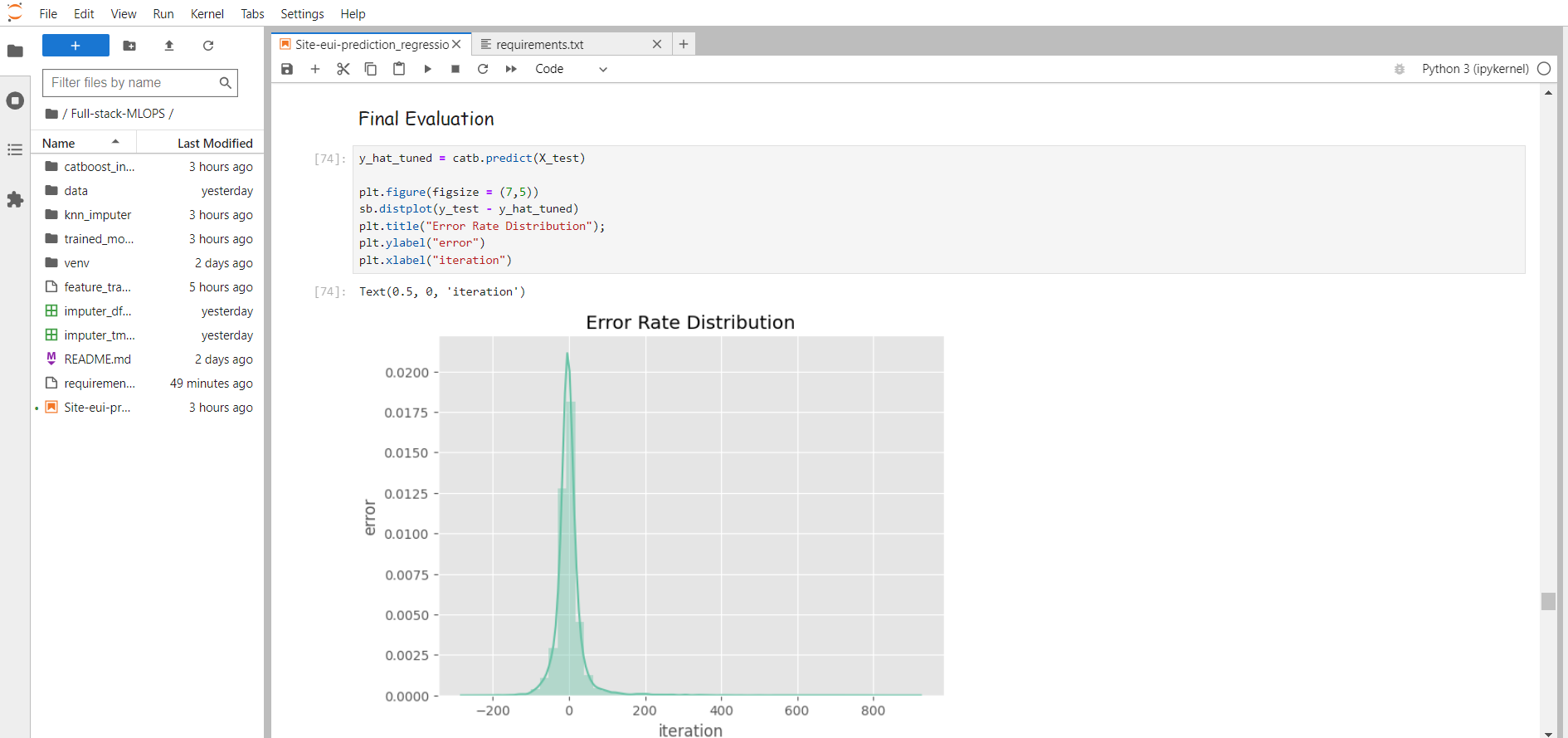
Further, I'm going to explain the model explainability in depth and how to interpret each fancy plot in shap.
10. Model Explainability using SHAP.
More on Model explainability
Now, let's make our model tell us why it makes certain predictions. SHAP values are like detectives explaining the evidence behind a conclusion. They break down which factors influence the decision, making it easier for us to trust and understand the machine's choices.
Before moving forward let's understand what shap values means and the nitty-gritty details behind each concept.
SHAP Model interpretation
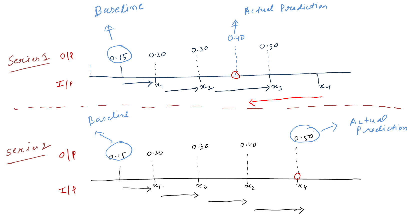
SHAP(i.e SHapley Additive exPlanations) leverages game theory to break down a prediction to measure the impact of each feature. A prediction can be explained by assuming that each feature value of the instance is a "player" in a game where the prediction is the prize money. The Shapley value, coined by Shapley, is a method for assigning payouts to players depending on their contribution to the total prize money amount.
If we all players(features) collaborate, how do we divide the payoff (Prediction)?
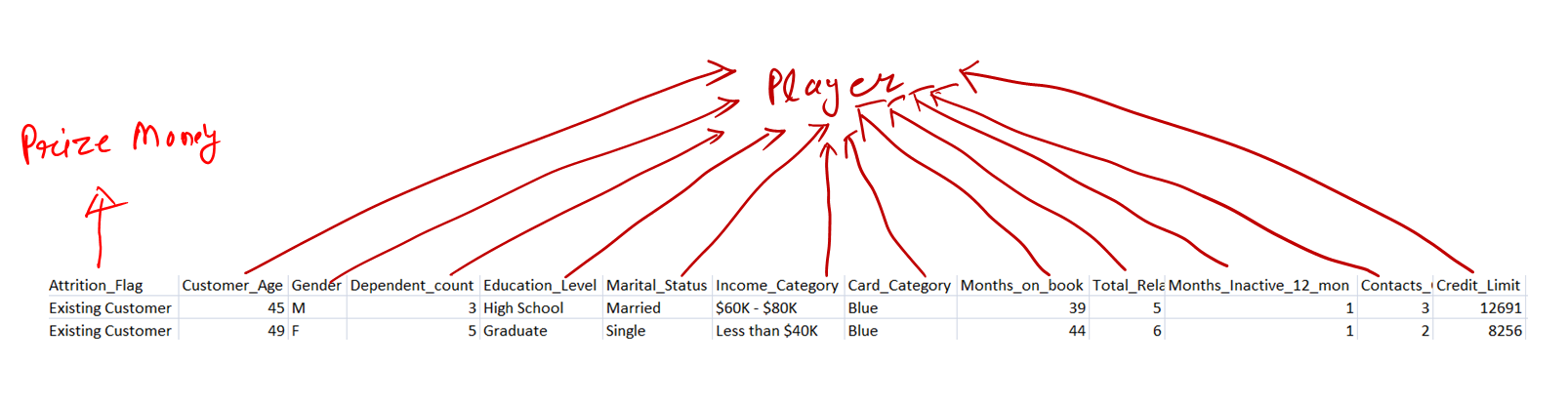
Compute Shapley value as the average: Average of each feature contribution over all possible feature ordering
For illustration purpose i have shown only two such series to understand the feature impact on prediction but in practice it will have 4! series for data containing 4 features = 24 possible series
What is Shapley values
Shapley values - Tells us how to fairly distribute the "Prize money" among the players (features).
SHAP values show "How much has each feature value contributed to the prediction compared to the average prediction?"
Shap value interpretation
Let's Understand each plot in-detail applied over the site_eui prediction dataset with catboost and random_forest model.
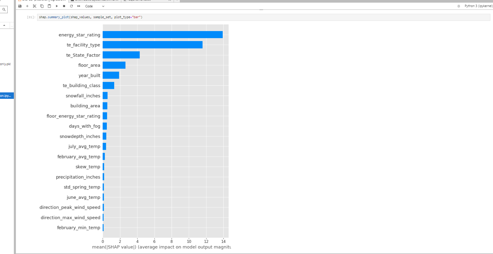
Bar Plot:
- As the problem we are solving is a regression problem, hence in our case bar plot indicates the feature importance based on how much it has contributed to the target model prediction. Our target is site_eui, so energy_star_rating, facility_type, state factor contributed a lot rather than temperature, wind-speed and fog etc.
Beeswarm Plot:
The summary plot combines feature importance with feature effects. The color represents the value of the feature from low to high. the dots in the plot represent the datapoints related to each feature and it's contribution to the prediction.
The features are ordered based on their mean shap values. red color represents high feature value and blue color represents lower feature value. the samples/datapoints on the right side of the y-axis represents positive impact on the prediction & datapoints on the left side represents negative impact on the prediction.
From the below plot, the energy_star_rating feature is more important for the prediction, and lower values of energy_star_rating are making a higher impact on prediction.
The more the spread of each feature on the x-axis, the more significant those features will be.
This plot gives an overall general idea about the feature impact.
This plot is made of many dots. Each dot has three characteristics:
Vertical location shows what feature it is depicting
Color shows whether that feature was high (RED Color) or low (BLUE Color) for any row of the dataset
Horizontal location of dots shows whether the effect of that value caused a higher or lower prediction. Negative shapley value will reduce the prediction probability and Positive shapley will increase prediction probability.

-
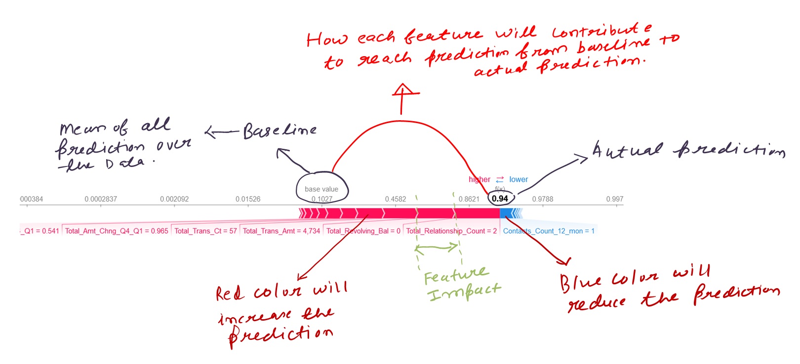
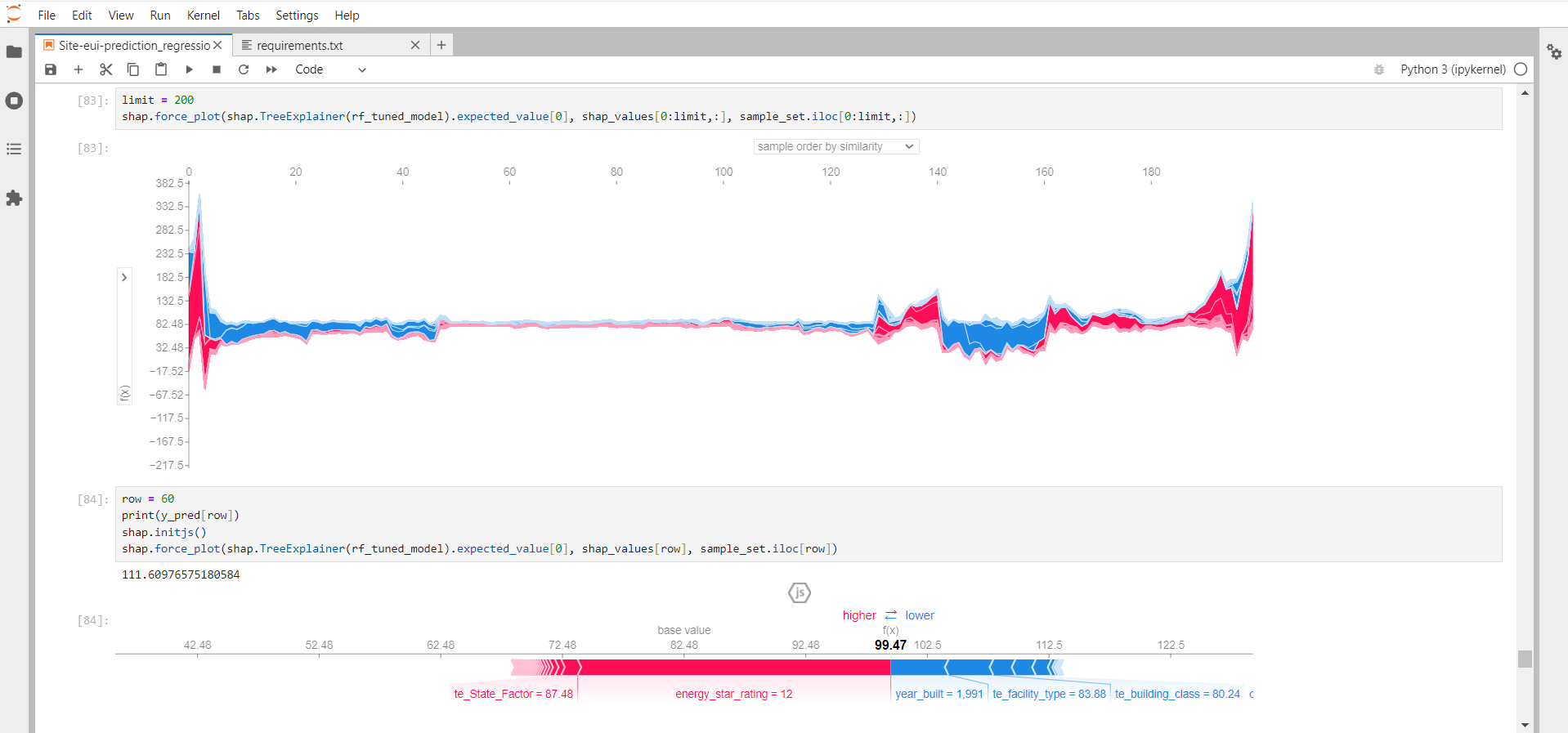
Force plots help to analyze the impact of each datapoint/sample on the prediction. This plot helps us to analyse the reason behind getting the predicted value=111.60 as per the below plot.
The first plot is a stacked force_plot
The second plot below can be interpreted for a single prediction. higher the width greater the impact it makes on the
prediction. from below energy_star_rating and year_built contributed largely to predict the 60th datapoint prediction as 111.60. the values in front of the feature represent datapoint values in the dataset.
Red arrows represent feature effects (SHAP values) that drives the prediction value higher while blue arrows are those effects that drive the prediction value lower. Each arrow’s size represents the magnitude of the corresponding feature’s effect. The “base value” (see the grey print towards the upper-left of the image) marks the model’s average prediction over the training set. The “output value” is the model’s prediction: probability 0.94. The feature values for the largest effects are printed at the bottom of the plot. Overall, the force plot provides an effective summary for this prediction.
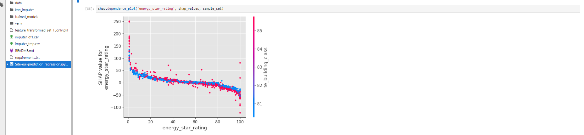
Dependence Plot:
The dependence plot represents the effect of a single datapoint across whole dataset.
SHAP dependence plots show the effect of a single feature across the whole dataset. They plot a feature's value vs. the SHAP value of that feature across many samples. SHAP dependence plots are similar to partial dependence plots, but account for the interaction effects present in the features, and are only defined in regions of the input space supported by data. The vertical dispersion of SHAP values at a single feature value is driven by interaction effects, and another feature is chosen for coloring to highlight possible interactions.
Each dot represents a row of the data.
The horizontal location is the actual value from the dataset, and the vertical location shows what having that value impacted prediction.
The Vertical dispersion at a single value of Total_Trans_Ct represents interaction effects with other features. To help reveal these interactions dependence_plot automatically selects another feature for coloring.
To understand how a single feature effects the output of the model we can plot the SHAP value of that feature vs. the value of the feature for all the examples in a dataset. Since SHAP values represent a feature's responsibility for a change in the model output, the plot above represents the change in site_eui probability as energy_star_rating changes.
As the energy_start_rating increases the site_eui prediction will decrease
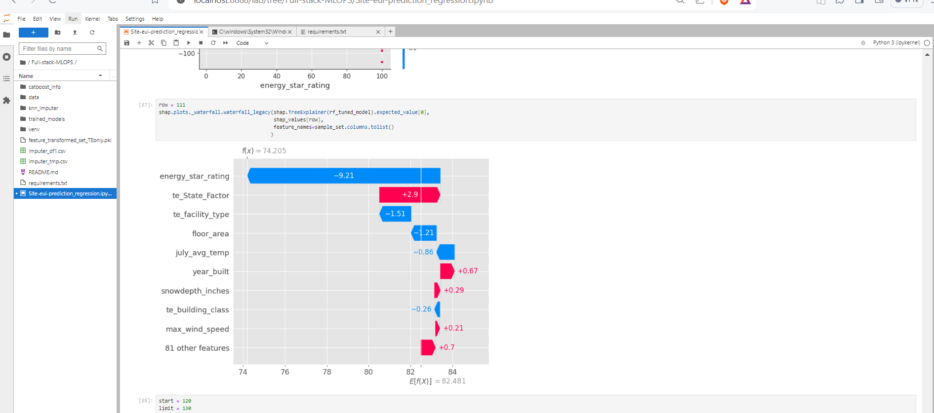
Waterfall Plot
Waterfall plot gives us the idea about the single datapoint contribution to the prediction. how each feature has contributed for making the prediction of 111th datapoint to be 74.205.
From the below plot it seems that energy_star_rating lower values made significant amount of impact on the prediction than higher values.
This graph may alter based on the datapoint/sample we are concern about.
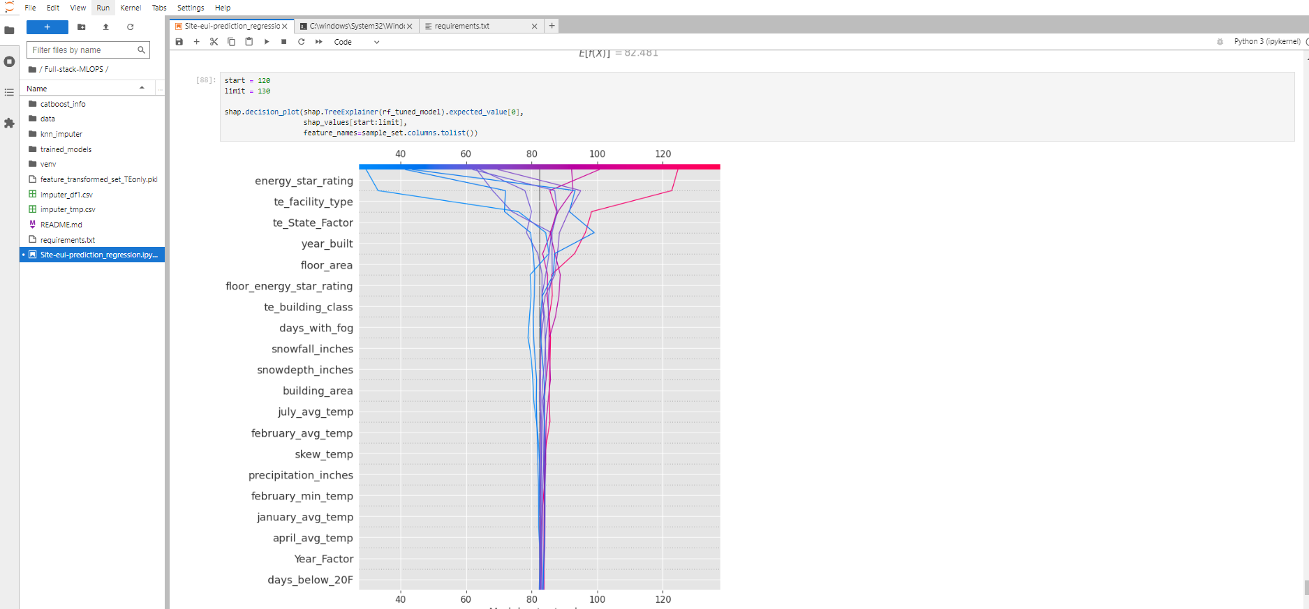
-
Decision plots offer a detailed view of a model’s inner workings; that is, they show how models make decisions.
There are several use cases for a decision plot.
  1) Show a large number of feature effects clearly.
  2) Visualize multioutput predictions.
  3) Display the cumulative effect of interactions.
  4) Explore feature effects for a range of feature values.
  5) Identify outliers.
  6) Identify typical prediction paths.
  7) Compare and contrast predictions for several models.
Interpretation of the below plot:
- The decision plot’s straight vertical line marks the model’s base value. The colored line is the prediction. Feature values are printed next to the prediction line for reference. Starting at the bottom of the plot, the prediction line shows how the SHAP values (i.e., the feature effects) accumulate from the base value to arrive at the model’s final score at the top of the plot. (Roughly speaking, this is similar to a statistical linear model where the sum of effects, plus an intercept, equals the prediction.) Decision plots are literal representation of SHAP values, making them easy to interpret.
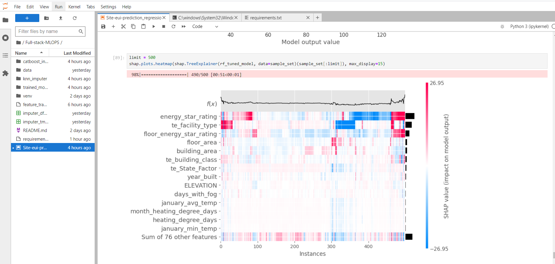
-
The width of the black bar on the right-hand side shows the global importance of each feature.
The heatmap plot is designed to show the population structure of a dataset using supervised clustering and a heatmap. Supervised clustering involves clustering the data points by their explanations and not by their original feature values. In a heatmap plot from shap, the x-axis is the instances, and the y-axis is the model inputs while the shap values are encoded on the color scale.
Hurrayyyy! You've just crafted your own machine learning masterpiece. By mastering each step, you've transformed raw data into powerful predictions. Remember, it's not about memorizing fancy words but understanding the story your data tells.
In the next article, I'm going to explain kfp-pipelines. How to build a sample kfp pipeline and each component of kfp in detail.
If you like these articles and wanted more such articles on AI, Data science, mlops, genAI on your feed daily, make sure to subscribe and follow me, connect with me on linkedin, github, kaggle.
Let's learn and Grow Together!!! Happy Learning:)


